Finite element calculations
This page solves a scalar Poisson problem. The key convention is that finite-element quadrature points are stored in the particle array: after update! fills the physical quadrature measures and basis data, the same @P2G and @P2G_Matrix macros used for MPM assemble finite-element vectors and matrices.
For quadrature point q in cell c, define a particle p by
\[\bm{x}_p = \bm{x}_c(\bm{\xi}_q), \qquad V_p = \omega_q \left|\det \bm{J}_c(\bm{\xi}_q)\right|.\]
Then a particle sum is the usual FEM quadrature rule:
\[\sum_p f(\bm{x}_p) V_p = \sum_c \sum_q f(\bm{x}_c(\bm{\xi}_q)) \omega_q \left|\det \bm{J}_c(\bm{\xi}_q)\right|.\]
The particle arrays in this page store fixed Gauss points, not moving MPM material points. With that convention, V[p] is the integration weight and the transfer macros become assembly loops.
Poisson Problem
Problem Setting
Solve
\[-\Delta u = 1 \quad \text{in } \Omega, \qquad u = 0 \quad \text{on } \Gamma_{\mathrm{outer}}, \qquad \nabla u \cdot \bm{n} = 1 \quad \text{on } \Gamma_{\mathrm{hole}},\]
where Ω is a rectangular plate with a circular hole, Γ_outer is the outside rectangle, and Γ_hole is the circular hole.
Generating the Mesh
For simple structured domains, a finite-element mesh can be generated directly from a CartesianMesh:
mesh = FEMesh(CartesianMesh(0.1, (0, 1), (0, 1)))For more complex domains, prepare a .msh file with Gmsh and read it with readmsh. This example uses the mesh file docs/src/assets/plate_with_hole.msh, which contains a rectangular plate with a circular hole. The file contains three physical groups that match the problem notation:
domain: triangular cells for volume integration.outer_boundary: line cells on the outside rectangle.hole_boundary: line cells on the circular hole.
Load Gmsh before calling readmsh. Each physical group is returned as a mesh in the dictionary, keyed by its group name.
using Tesserae
using Gmsh
using LinearAlgebra

meshdir = joinpath(pkgdir(Tesserae), "docs", "src", "assets")
mshfile = joinpath(meshdir, "plate_with_hole.msh")
meshes = readmsh(mshfile; gmsh_argv=["-v", "0"]);

domain = meshes["domain"]
outer_boundary = meshes["outer_boundary"]
hole_boundary = meshes["hole_boundary"]

plot_gmsh_groups(domain, outer_boundary, hole_boundary)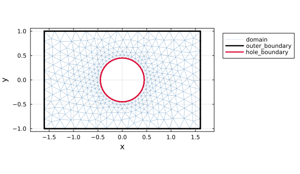
Plot helpers
import Plots

function segment_coordinates(mesh)
    xs = Float64[]
    ys = Float64[]
    for cell in cells(mesh)
        nodes = supportnodes(mesh, cell)
        for a in eachindex(nodes)
            i = nodes[a]
            j = nodes[mod1(a + 1, length(nodes))]
            push!(xs, mesh[i][1], mesh[j][1], NaN)
            push!(ys, mesh[i][2], mesh[j][2], NaN)
        end
    end
    xs, ys
end

function plot_gmsh_groups(domain, outer_boundary, hole_boundary)
    plt = Plots.plot(;
        aspect_ratio=:equal,
        legend=:outertopright,
        xlabel="x",
        ylabel="y",
        size=(620, 360),
        framestyle=:box,
    )
    xs, ys = segment_coordinates(domain)
    Plots.plot!(plt, xs, ys; color=:steelblue, linewidth=0.45, alpha=0.45, label="domain")
    xs, ys = segment_coordinates(outer_boundary)
    Plots.plot!(plt, xs, ys; color=:black, linewidth=2.5, label="outer_boundary")
    xs, ys = segment_coordinates(hole_boundary)
    Plots.plot!(plt, xs, ys; color=:crimson, linewidth=2.5, label="hole_boundary")
    plt
end
Quadrature Data
Use the domain physical group as the finite-element mesh. From the transfer macros, the objects have the same roles as in MPM: grid stores nodal fields, gauss_points is the point array, and weights connects each point to the grid nodes. gauss_points has one row per quadrature point and one column per cell.
GridProp = @NamedTuple begin
    x :: Vec{2, Float64}
    u :: Float64
    f :: Float64
end

GaussProp = @NamedTuple begin
    x :: Vec{2, Float64}
    V :: Float64
end

grid = generate_grid(GridProp, domain)
rule = generate_quadrature_rule(basis(domain))
gauss_points = generate_particles(GaussProp, domain, rule)
weights = generate_basis_weights(domain, size(gauss_points); name=Val(:N))

update!(weights, gauss_points, domain; measure=gauss_points.V)
3×722 BasisWeightArray:
Basis: Tesserae.Tri3()
Basis values: N, ∇NThe basis-weight array has the same nq × ncells shape as gauss_points. After update!, each entry stores the element-local basis data for one Gauss point: N[ip] and ∇N[ip] are the value and physical gradient of the basis function associated with local support index ip, and V[p] is the quadrature weight multiplied by the Jacobian measure. This is the same grid/particles/weights pattern used by MPM assembly, but the support nodes come from the finite-element cell connectivity instead of a moving particle search.
Assembly
For the domain terms in the weak form,
\[f_i = \int_\Omega N_i \, d\Omega \approx \sum_p N_i(\bm{x}_p) V_p, \qquad K_{ij} = \int_\Omega \nabla N_i \cdot \nabla N_j \, d\Omega \approx \sum_p \nabla N_i(\bm{x}_p) \cdot \nabla N_j(\bm{x}_p) V_p.\]
Those two terms are assembled directly with transfer macros:
K = create_sparse_matrix(domain; ndofs=1)

@P2G grid=>i gauss_points=>p weights=>ip begin
    f[i] = @∑ N[ip] * V[p]
end

@P2G_Matrix grid=>(i,j) gauss_points=>p weights=>(ip,jp) begin
    K[i,j] = @∑ ∇N[ip] ⋅ ∇N[jp] * V[p]
end
The Neumann condition on hole_boundary contributes a boundary integral to the right-hand side. Boundary meshes share the domain node numbering, so the contribution can be accumulated into the same grid.f field.
BoundaryGaussProp = @NamedTuple begin
    x :: Vec{2, Float64}
    dS :: Float64
    n :: Vec{2, Float64}
end

boundary_rule = generate_quadrature_rule(basis(hole_boundary))
hole_gauss_points = generate_particles(BoundaryGaussProp, hole_boundary, boundary_rule)
hole_weights = generate_basis_weights(hole_boundary, size(hole_gauss_points); name=Val(:N))

update!(
    hole_weights,
    hole_gauss_points,
    hole_boundary;
    measure=hole_gauss_points.dS,
    normal=hole_gauss_points.n,
)

neumann_flux(x, n) = 1.0

@P2G grid=>i hole_gauss_points=>p hole_weights=>ip begin
    f[i] = @∑ N[ip] * neumann_flux(x[p], n[p]) * dS[p]
end
Boundary Conditions
The outer boundary uses homogeneous Dirichlet data. The boundary values stay zero and only the free degrees of freedom are solved.
The solution grid.u is a nodal field. The plot below colors each triangular cell by the average of its nodal values and overlays the boundary groups.
boundary_nodes = supportnodes(outer_boundary)

dofmask = trues(1, size(grid)...)
dofmask[1, boundary_nodes] .= false

free = DofMap(dofmask)
free(grid.u) .= Symmetric(extract(K, free)) \ Array(free(grid.f))

plot_solution(domain, grid.u, outer_boundary, hole_boundary)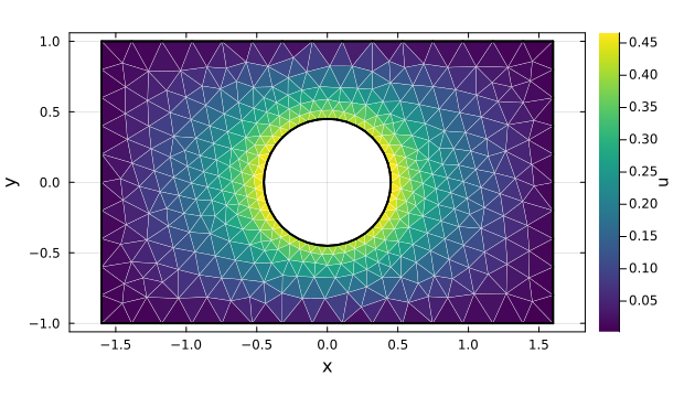
Solution plot helpers
import Plots

function plot_solution(mesh, u, outer_boundary, hole_boundary)
    shapes = Plots.Shape[]
    values = Float64[]

    for cell in cells(mesh)
        nodes = supportnodes(mesh, cell)
        push!(shapes, Plots.Shape([mesh[i][1] for i in nodes], [mesh[i][2] for i in nodes]))
        push!(values, sum(u[i] for i in nodes) / length(nodes))
    end

    plt = Plots.plot(
        shapes;
        fill_z=permutedims(values),
        color=:viridis,
        linecolor=:white,
        linewidth=0.25,
        colorbar_title="u",
        aspect_ratio=:equal,
        xlabel="x",
        ylabel="y",
        label=false,
        size=(620, 360),
        framestyle=:box,
    )
    bx, by = segment_coordinates(outer_boundary)
    Plots.plot!(plt, bx, by; color=:black, linewidth=1.8, label=false)
    bx, by = segment_coordinates(hole_boundary)
    Plots.plot!(plt, bx, by; color=:black, linewidth=1.8, label=false)
    plt
end
API
Tesserae.FEMesh — Type
FEMesh(shape, nodes, cellsupports)
FEMesh(cartesian_mesh)
FEMesh(shape, cartesian_mesh)
Create a finite-element mesh.
shape is the cell shape, nodes stores the nodal coordinates, and cellsupports stores the node indices of each cell. cells(mesh) iterates over cell indices, while supportnodes(mesh, cell) returns the nodes used by one cell.
The Cartesian constructors are convenience constructors for structured test meshes and examples. FEMesh(cartesian_mesh) uses the default first-order cell shape for the dimension: Line2, Quad4, or Hex8. Passing an explicit shape allows triangular, tetrahedral, and higher-order cells to be generated from the Cartesian grid.
FEMesh is used by the finite-element workflow. Use generate_particles to create quadrature points, generate_basis_weights to create element-local basis storage, and update! to fill the element-local basis data.
Tesserae.generate_field_meshes — Function
generate_field_meshes(meshes[, order])Construct consistently numbered field meshes from geometry meshes that share one node array. Maximum-dimensional cells define the field nodes; lower-dimensional meshes must match their faces or edges.
Omit order, or pass the order already used by every shape, to preserve the geometry shapes. Pass Order(1) to replace them with first-order shapes. The returned meshes share a compact view of the geometry nodes. Tuple order and dictionary keys are preserved.
Tesserae.supportnodes — Method
supportnodes(mesh::FEMesh)
supportnodes(mesh::FEMesh, cell::Int)
Return the sorted node indices used by mesh, or the local support node indices of cell.
Tesserae.update! — Method
update!(weights::BasisWeightArray{<:Shape}, points::QuadraturePoints, fieldmesh::FEMesh; geometry=fieldmesh, measure=nothing, normal=nothing)Evaluate the basis of fieldmesh using the quadrature rule stored in points, with geometry defining the physical mapping. geometry defaults to fieldmesh. If they differ, the meshes must describe the same cells in the same order and orientation.
For full-dimensional cells, weights stores basis values and physical gradients. For boundary cells, it stores basis values. measure receives the physical quadrature measure, and normal receives boundary unit normals.
Tesserae.readmsh — Function
readmsh(filename::AbstractString; gmsh_argv=String[], reorient_boundary=false)Read a Gmsh .msh file.
This method is provided by the Gmsh extension. Load Gmsh before calling it:
using Tesserae
using Gmsh

meshes = readmsh("mesh.msh")
Returns a Dict{String,FEMesh} keyed by physical group name. Each physical group is read as one FEMesh and must contain exactly one supported element shape. Unnamed physical groups use keys of the form "physical_group[dim,tag]".
Pass reorient_boundary=true to reorder boundary cells that match exactly one volume face to follow the outward volume face orientation. Boundary cells that do not match a volume face, or match multiple volume faces, are left unchanged and reported with a warning.