Isogeometric analysis calculations

Experimental

IGA support is experimental and its API may change.

This page solves a scalar heat-conduction problem on a NURBS patch. The assembly flow is the same as in Finite element calculations: quadrature points are stored in the particle array, update! fills the basis values and physical quadrature measures, and @P2G_Matrix assembles the global matrix.

The difference is the geometric and discrete basis. An IGAMesh uses NURBS control points as grid entries, and the unknown grid.u stores control coefficients, not nodal values. A field value inside the patch is evaluated by the same rational basis functions that describe the geometry.

Quarter Annulus

Problem Setting

Solve

\[-\Delta u = 0 \quad \text{in } \Omega, \qquad u = 1 \quad \text{on } r = r_i, \qquad u = 0 \quad \text{on } r = r_o.\]

The radial sides are left as natural boundaries:

\[\nabla u \cdot \bm{n} = 0 \quad \text{on } \theta = 0,\ \theta = \pi/2.\]

This problem has the analytic solution

\[u(r) = \frac{\log(r_o / r)}{\log(r_o / r_i)}.\]

The circular boundaries are represented exactly by rational quadratic NURBS curves.

Building the NURBS Patch

Create the quarter annulus from two circular arcs and two radial line segments. Tesserae.NURBS.coons_patch blends those four boundary curves into one tensor-product surface. The first parametric direction follows the angle, and the second direction follows the radius.

using Tesserae
using LinearAlgebra
NURBS = Tesserae.NURBS

ri = 1.0
ro = 2.0
center = Vec(0.0, 0.0)

inner_curve = NURBS.arc(center, ri, 0.0, π / 2)
outer_curve = NURBS.arc(center, ro, 0.0, π / 2)
radial0_curve = NURBS.line(Vec(ri, 0.0), Vec(ro, 0.0))
radial1_curve = NURBS.line(Vec(0.0, ri), Vec(0.0, ro))

surface = NURBS.coons_patch(inner_curve, outer_curve, radial0_curve, radial1_curve)
surface = NURBS.elevate(surface, (NURBS.quadratic, NURBS.quadratic))
surface = NURBS.refine(surface, (20, 8))

mesh = IGAMesh(surface)

inner_boundary = boundaries(mesh, 1, 2, -1)
outer_boundary = boundaries(mesh, 1, 2, +1)

plot_patch(surface)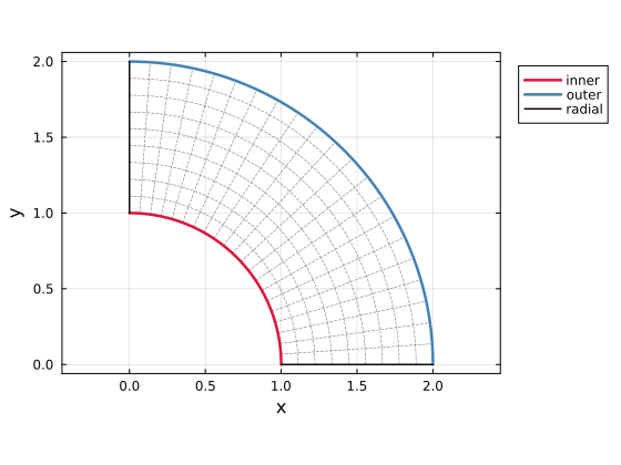

Plot helpers

import Plots

function plot_line!(plt, points; kwargs...)
    xs = [point[1] for point in points]
    ys = [point[2] for point in points]
    Plots.plot!(plt, xs, ys; kwargs...)
end

function patch_line(surface, direction, value; n=120)
    other_direction = 3 - direction
    lower, upper = Tesserae.NURBS.domain(surface, other_direction)
    if direction == 1
        [Tesserae.NURBS.evaluate(surface, Vec(value, η)) for η in range(lower, upper; length=n)]
    else
        [Tesserae.NURBS.evaluate(surface, Vec(ξ, value)) for ξ in range(lower, upper; length=n)]
    end
end

function patch_curve(surface, direction, side; n=120)
    lower, upper = Tesserae.NURBS.domain(surface, direction)
    fixed = side == -1 ? lower : upper
    patch_line(surface, direction, fixed; n)
end

function knot_values(surface, direction)
    lower, upper = Tesserae.NURBS.domain(surface, direction)
    values = unique(Tesserae.NURBS.knots(surface, direction))
    filter(ξ -> lower ≤ ξ ≤ upper, values)
end

function plot_knot_lines!(plt, surface; n=80)
    for ξ in knot_values(surface, 1)
        plot_line!(plt, patch_line(surface, 1, ξ; n); color=:gray, linestyle=:dash, linewidth=0.6, label=false)
    end
    for η in knot_values(surface, 2)
        plot_line!(plt, patch_line(surface, 2, η; n); color=:gray, linestyle=:dash, linewidth=0.6, label=false)
    end
    plt
end

function plot_patch(surface)
    plt = Plots.plot(;
        aspect_ratio=:equal,
        xlabel="x",
        ylabel="y",
        size=(560, 420),
        framestyle=:box,
        legend=:outertopright,
    )

    plot_knot_lines!(plt, surface)
    plot_line!(plt, patch_curve(surface, 2, -1); color=:crimson, linewidth=2.5, label="inner")
    plot_line!(plt, patch_curve(surface, 2, +1); color=:steelblue, linewidth=2.5, label="outer")
    plot_line!(plt, patch_curve(surface, 1, -1); color=:black, linewidth=1.4, label="radial")
    plot_line!(plt, patch_curve(surface, 1, +1); color=:black, linewidth=1.4, label=false)
    plt
end

Quadrature Data

From the transfer macros, the objects have the same roles as in MPM and FEM: grid stores the control-point fields, gauss_points is the point array, and weights connects each Gauss point to the active control points.

GridProp = @NamedTuple begin
    x :: Vec{2, Float64}
    u :: Float64
    f :: Float64
end

GaussProp = @NamedTuple begin
    x :: Vec{2, Float64}
    u :: Float64
    V :: Float64
end

grid = generate_grid(GridProp, mesh)
rule = generate_quadrature_rule(basis(mesh))
gauss_points = generate_particles(GaussProp, mesh, rule)
weights = generate_basis_weights(mesh, size(gauss_points); name=Val(:N))

update!(weights, gauss_points, mesh; measure=gauss_points.V)

9×189 BasisWeightArray: 
  Basis: IGABasis{2, Tuple{Quadratic, Quadratic}}((Quadratic(), Quadratic()))
  Basis values: N, ∇N

After update!, N[ip] and ∇N[ip] are the rational basis value and physical gradient associated with local support index ip. The value V[p] is the quadrature weight multiplied by the physical Jacobian measure.

Assembly

The weak form only has the stiffness term:

\[K_{ij} = \int_\Omega \nabla N_i \cdot \nabla N_j \, d\Omega \approx \sum_p \nabla N_i(\bm{x}_p) \cdot \nabla N_j(\bm{x}_p) V_p.\]

As in the FEM example, the global matrix is assembled with @P2G_Matrix:

K = create_sparse_matrix(mesh; ndofs=1)

@P2G_Matrix grid=>(i,j) gauss_points=>p weights=>(ip,jp) begin
    K[i,j] = @∑ ∇N[ip] ⋅ ∇N[jp] * V[p]
end

Boundary Conditions

The inner and outer circular boundaries use Dirichlet data. Because IGA uses control coefficients, constant boundary data are imposed by setting all control coefficients on that boundary to the constant value. The radial sides require no extra assembly for the homogeneous Neumann condition.

inner_nodes = supportnodes(inner_boundary)
outer_nodes = supportnodes(outer_boundary)
boundary_nodes = union(inner_nodes, outer_nodes)

grid.u[inner_nodes] .= 1.0
grid.u[outer_nodes] .= 0.0

dofmask = trues(1, size(grid)...)
dofmask[1, boundary_nodes] .= false

free = DofMap(dofmask)
rhs = grid.f - K * grid.u
free(grid.u) .= Symmetric(extract(K, free)) \ Array(free(rhs));

Verification

The analytic solution depends only on the physical radius. Transfer the solved control coefficients to the existing Gauss points and compute the maximum absolute error over those points.

exact_solution(x) = log(ro / norm(x)) / log(ro / ri)

@G2P grid=>i gauss_points=>p weights=>ip begin
    u[p] = @∑ N[ip] * u[i]
end

max_error = maximum(abs, gauss_points.u .- exact_solution.(gauss_points.x))

round(max_error; sigdigits=3)

2.39e-5

plot_solution(surface, grid.u)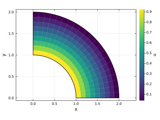

Solution helpers

function plot_solution(surface, u)
    solution = Tesserae.NURBS.ControlNet(
        surface.axes,
        map(value -> Vec(value), reshape(u, size(surface.points))),
        surface.weights,
    )
    ξs = knot_values(surface, 1)
    ηs = knot_values(surface, 2)
    shapes = Plots.Shape[]
    values = Float64[]

    for j in 1:(length(ηs)-1), i in 1:(length(ξs)-1)
        corners = (
            Vec(ξs[i], ηs[j]),
            Vec(ξs[i+1], ηs[j]),
            Vec(ξs[i+1], ηs[j+1]),
            Vec(ξs[i], ηs[j+1]),
        )
        points = map(ξ -> Tesserae.NURBS.evaluate(surface, ξ), corners)
        push!(shapes, Plots.Shape([point[1] for point in points], [point[2] for point in points]))
        push!(values, sum(only(Tesserae.NURBS.evaluate(solution, ξ)) for ξ in corners) / length(corners))
    end

    plt = Plots.plot(
        shapes;
        fill_z=permutedims(values),
        color=:viridis,
        linecolor=:white,
        linewidth=0.05,
        colorbar_title="u",
        aspect_ratio=:equal,
        xlabel="x",
        ylabel="y",
        label=false,
        size=(560, 420),
        framestyle=:box,
    )
    plot_line!(plt, patch_curve(surface, 2, -1); color=:black, linewidth=1.5, label=false)
    plot_line!(plt, patch_curve(surface, 2, +1); color=:black, linewidth=1.5, label=false)
    plot_line!(plt, patch_curve(surface, 1, -1); color=:black, linewidth=1.5, label=false)
    plot_line!(plt, patch_curve(surface, 1, +1); color=:black, linewidth=1.5, label=false)
    plt
end

API

IGA

Tesserae.IGAPatch — Type

IGAPatch(degrees, knot_vectors, controlpoint_ids)

Define a tensor-product IGA patch.